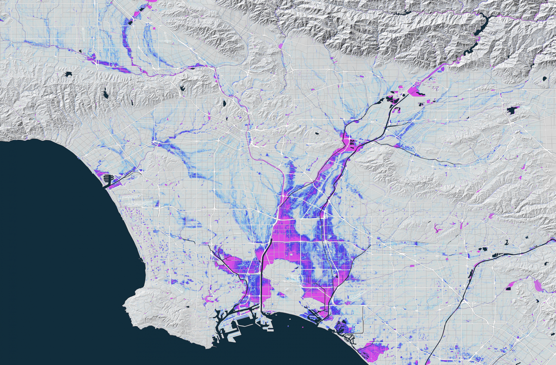
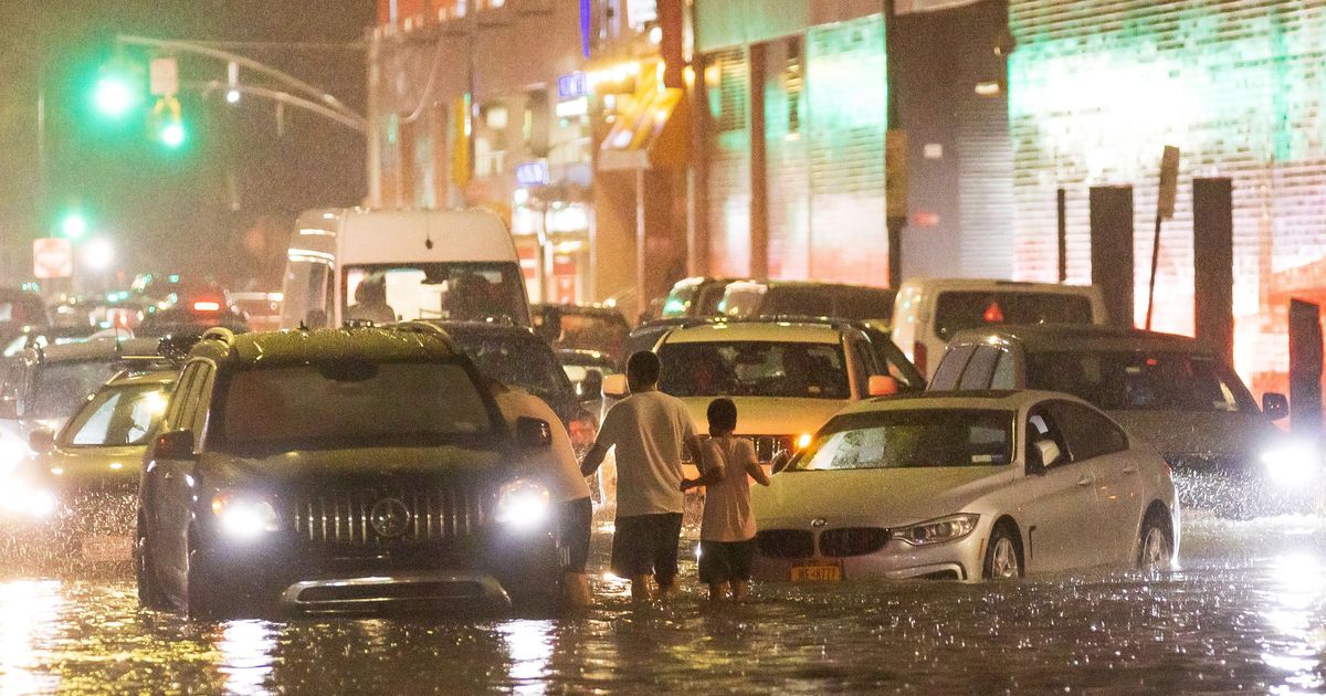
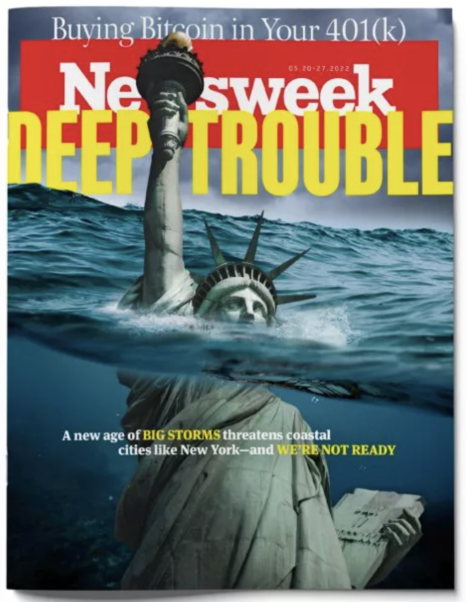
MATLAB CODES

Matlab is an integrated numerical analysis package that makes it very easy to implement computational modeling codes. The vast majority of students taking my classes have either little or rusty programming experience, and the minimal overhead and integrated graphics capabilities of Matlab makes it a good choice for beginners.

On this page are a few basic codes that may be of interest to students of computational hydraulics. These codes have been developed for instructional and research purposes, and have been shared with students of my graduate courses in the past.

1D Wet-Bed Shallow-Water Solver

Here is a zip file containing a set of Matlab files that implement a Godunov-type finite volume scheme for solving the 1D shallow-water equations. The equations solved by the code are depth-integrated, as opposed to cross-sectionally integrated, and flow resistance is ignored. As such, the code has little practical value. Further, this particular code is not suited to problems involving a dry bed. It should only be run in problems where all cells are wetted with a least a millimeter or so of water. These simplifications are made to emphasize the simplicity of the code. The problem of wetting and drying requires a number of if - then type statements, to avoid division by zero among other things, and this detracts from the overall simplicity of the code. For instructional purposes, this is paramount.

To execute this code using Matlab, copy all of the .m files into a common directory and execute the script entitled fvm1d.m at the command prompt. This is a Matlab script file that contains the main block of code; all others are Matlab function files that act as subroutines.

The code can be implemented in either a first-order or second-order accurate mode. In first-order mode, the code only uses the fluxes.m , solver.m and corrector.m function files. The first of these sweeps over all edges or faces in the 1D grid to compute mass and momentum fluxes, the second implements Roe's approximate Riemann solver with a critical flow fix recommended by Bram van Leer, and the third advances the solution from the n to the n+1 time levels. The remaining function files are used for second-order accuracy, for example predictor.m advances the solution from the n to the n+1/2 time level by solving the primitive form ofthe 1D shallow-water equations, and the limiter.m and limit.m files are used for slope limiting purposes. A parameter can be changed in fvm1d.m to switch between various slope limiters such as minmod, superbee, van Leer, van Albada and double minmod.

In my class, I encourage students to begin by running the code as-is, to experiment with different initial conditions, grid spacings, and time steps, and then to implement bigger changes. For example, students should try to implement different boundary conditions, account for flow resistance, account for dry-bed problems, and extend the model to 2D.

2D Wet-Bed Shallow-Water Solver

Here is a zip file containing a set of Matlab files that implement a numerical solution to the 2D shallow-water equations on a Cartesian grid. The numerical method is a first-order accurate Godunov-type finite volume scheme that utilizes Roe's approximate Riemann solver. Like the 1D code above, the 2D code is highly simplistic: It is set up to model long wave action in a square tank with a flat bottom and no flow resistance. It wouldn't take much effort to update the model for variable topography and flow resistance. In fact, I recommend it to students in graduate courses on hydraulic modeling. It would be a worthwhile homework exercise. Please be warned that the code runs slowly. The same logic coded in Fortran would run much, much faster.

To execute this code using Matlab, copy all of the .m files into a common directory and execute the script entitled fvm2d.m at the command prompt. This is a Matlab script file that contains the main block of code; all others are Matlab function files that act as subroutines.

A worthwhile exercise for students would be to extend this code to second-order accuracy. The 1D solver above can be used as a guide, and the numerical methods are comprehensively described Bradford and Sanders (2002)
.

2D Wet-Bed Shallow-Water Solver Using Local Time Stepping

Here is a zip file containing a set of Matlab files very similar to the 2D solver above, except that the local time-stepping scheme described in Sanders (2008) is implemented.

To execute this code using Matlab, copy all of the .m files into a common directory and execute the script entitled fvm2d_lts.m at the command prompt. This is a Matlab script file that contains the main block of code; all others are Matlab function files that act as subroutines.

Experiment with the number of LTS levels (e.g., 1, 2, 3 and 4) and examine how both run-time and the accuracy change. Using LTS_levels=1 corresponds to a conventional global time stepping scheme. This simple application shows that there are benefits to using LTS even in problems with a uniform grid resolution.

1D Gradually Varied Flow Solver

Here is a zip file containing a pair of Matlab files that solve the steady state gradually varied flow equation using Matlab's built-in Runge Kutta solver, ode45 . There are only two Matlab files. The first, gvf.m contains the main program block and should be executed at the command prompt, and the second, gvfrhs.m is a function file that evaluates the right-hand side of the gradually varied flow ODE. The code is set up to predict a sub-critical flow profile, starting at the downstream end of a sloping channel and integrating upstream, in the negative x direction. For supercritical flow profiles, integration should proceed in the positive x direction and this can be accomplished with minor modifications to the code.

Unstructured Grid Model for 2D Scalar Transport

Here is a zip file containing a Matlab program to solve the 2D advection equation on an unstructured grid. This program was developed to introduce students to unstructured grids, and those seeking an introduction to unstructured grids might find it worthwhile to run. This can be done by unzipping the folder and executing the unstructured.m script. The spatial domain is a box and an analytical model for the fluid velocity is used to produce a swirling motion. The grids were generated using Triangle. Note that the transport solver sweeps over all cells and updates the solution using a first order accurate scheme. Upon updating the solution a cell, the solver sweeps over the three neighboring edges to compute the necessary fluxes. A more efficient approach is to first sweep over all faces to compute fluxes globally, and then to sweep over cells to update the solution to the new time level. Triangle outputs a list of edges to support this approach using the -e option. Begnudelli and Sanders (2006) describe bookeeping conventions that we've used with unstructured grids.

Particle Tracking Model for 2D Diffusion

Here is a zip file containing a Matlab program to solve the 2D diffusion equation using a random-walk particle tracking method. The solution corresponds to an instantaneous load of particles at the origin at time zero. The program was designed to help students understand the diffusion process and as an introduction to particle tracking methods. When executed, the randomwalk.m program will track the position of N particles and output an animation of graphs that display the particle distribution in the form of :(a) particle position, (b) particle concentration versus x , (c) particle concentration versus y , and (d) the 2D particle concentration. Particle tracking codes such as these can be integrated into larger envirionmental simulation codes for unique analyses not possible with continuum approaches. For example, Arega and Sanders (2004) integrated particle tracking into a flow and transport model for tidal wetlands to study dispersion.

Particle Tracking Model for 2D Taylor Dispersion

Here is a script file taylor.m containing a Matlab program to solve the advection diffusion equation in a 2D channel flow with a parabolic velocity distribution (laminar flow). The solution corresponds to an instantaneous load of particles along an x=0 line at time zero. The program was designed to help students understand Taylor dispersion, which results from the combined effects of cross-channel diffusion and longitudinal advection by a velocity distribution that varies with y . When executed, the taylor.m program will track the position of N particles and output an animation of graphs that display the particle distribution in the form of :(a) particle position in a moving coordinate system , x'=x-Vt , (b) particle concentration versus x-Vt , (c) variance of the particle distribution in the x direction versus time. Taylor's theory predicts that the variance will grow linearly with time after an initial adjustment period, and this can be seen clearly in (c).


RETURN TO MAIN PAGE